Eulerian Fluid Simulation [Part 1]

Eulerian vs Lagrangian Fluid Simulation

There are two main schools of thought for simulating fluids. The Lagrangian approach simulates a large number of particles to approximate fluid molecules whereas the Eulerian approach divides the simulation space into grid cells at which we keep track of different fluid properties such as velocity, pressure, and temperature.

The Lagrangian approach can easily simulate small-scale effects since it measures properties of the fluid at each individual particle. To mimic this level of detail, the Eulerian approach would need to increase the resolution of the grid as fluid effects smaller than the size of a grid cell cannot be accurately represented.

In contrast, the Eulerian approach can simulate large-scale effects significantly faster as it only needs to maintain the one value per property in each grid cell whereas the Lagrangian approach would need to simulate a large quantity of particles to fill the each grid cell in order to produce the same effect.

As a midground, there are hybrid models that use Eulerian grids overall with Lagrangian particles near the surface where there many small-scale fluid effects. Alternatively, non-uniform adaptively sampled grids can similarly reduce the computational workload while maintaining high levels of resolution where needed.

For the remainder of this article, we'll be focusing on the Eulerian approach for incompressible fluids. This article can be seen as my abridged version of Robert Bridson's notes / textbook¹ and draws some intuition and ideas from Foster and Metaxas.²

Notation

Following the standard notation of fluid simulation texts and literature, we denote velocity to be the vector \(\vec{u} = (u, v, w)\) whose components correspond to the velocity components in the \(x, y, z\) directions respectively. Pressure will be denoted as \(p\) and we'll denote any other quantity we keep track of in the grid as \(q\).

We also define \(\rho\) to be the density of the fluid, \(\eta\) to be the dynamic viscosity coefficient and \(\nu = \frac{\eta}{\rho}\) to be the kinematic viscosity.

Behavior of Fluid

The first question we can ask ourselves is how do fluids behave? Or more importantly, what forces control the behavior of fluids?

• The immediate answer would be gravity (as well as any other external forces acting on the fluid) that exerts a downward force on the fluid.³
• We also have pressure as fluids gradually move from areas of high pressure to areas of low pressure.
• And lastly, we have viscosity which resists deformation of the fluid. Notice that if fluid moves uniformly locally, then that local region would not have any deformation. Therefore, viscosity can be seen as a "force" that resists non-uniform local movement.

Material Derivative

Given that we're measuring quantities on the grid, we need to know how they change in order to update their values. Namely, the question we want to answer is what is the rate of change of a fluid property at a given location over time?

Naively, we would think that this would simply be the time derivative of the fluid property, but this does not account for fluid movement. Imagine that at a grid point \(x\), we have some fluid particles \(f^0\). After we advance one time step in the simulation, barring zero velocity at \(x\), those fluid particles should have moved to a new location and other fluid particles \(f^1\) may have taken its place at \(x\). As a result, the value of the measured fluid property at \(x\) is now that of the particles \(f^1\).

Combining both the time derivative of the property and the fluid flow, we obtain the material derivative, denoted with a capital D, which is defined as follows for a property \(q\) :

$$\frac{Dq}{Dt} = \frac{\partial q}{\partial t} + u \frac{\partial q}{\partial x} + v \frac{\partial q}{\partial y} + w \frac{\partial q}{\partial z}$$

By multiplying the spatial derivatives of \(q\) with the fluid velocity, we additional account for how \(q\) changes as fluid moves through the velocity field \(\vec{u}\). We can also write this more succinctly as:

$$\frac{Dq}{Dt} = \frac{\partial q}{\partial t} + \vec{u} \cdot \nabla q$$

Putting Everything Together

Viewing the material derivative of velocity as acceleration, we want to see how it's affected by the three "forces" we described earlier so that we can update the velocity field every step.

• In the case of gravity, we accelerate the \(y\) component of \(\vec{u}\) by the gravitational constant \(g\) as per usual.
• For pressure, we want to have an acceleration applied to \(\vec{u}\) that pushes it towards lower pressure regions. Looking a particular point, we have that the gradient of the pressure yields the direction of steepest ascent. In order to get desired descent direction, we simply have to negate it.
• For viscosity, we want to resist large differences in velocity in local regions. The Laplacian operator, \(\nabla^2\), does exactly that when applied to the velocity field. See the appendix section for intuition and review of the Laplacian operator.

To convert the pressure and viscosity into a force, we integrate these values over the volume and the gravitational force is the usual, \(mg\). Putting everything together, we have:

$$m\frac{D\vec{u}}{Dt} = - V , \nabla p + mg + \eta V , \nabla^2 \vec{u}$$

Dividing by volume and then by density, we are left with the first of the Navier-Stokes equations:

$$\frac{D\vec{u}}{Dt} = - \frac{1}{\rho} \nabla p + g + \nu \nabla^2 \vec{u}$$

Incompressibility

The second of the Navier-Stokes equations deals with the incompressibility constraint of fluids. Namely, we want to preserve the volume as we simulate it. This boils down to wanting the amount of fluid that enters a given region to be equal to the amount of fluid that leaves it.

Recalling calculus, this is equivalent to wanting the integral of the normal component of the velocity over the boundary of any given region \(\Omega\) to be zero:

$$\iint_{\partial\Omega}\vec{u}\cdot\hat{n} = 0$$

Using the fundamental theorem of calculus we have that:

$$\iiint_\Omega\nabla\cdot\vec{u} = 0$$

Since this has to hold for any region \(\Omega\), we have that:

$$\nabla\cdot\vec{u} = 0$$

MAC Grid

Imagine first that we put the velocity values in the center of the grid cells and approximate the derivative with central differencing. Central differencing is preferred over forwards or backwards differencing because it doesn't have a left or right bias and the error term is \(O(n^2)\) rather than \(O(n)\). However, it comes with a small problem:

$$u_i' \approx \frac{u_{i + 1} - u_{i - 1}}{2\Delta x}$$

Notice that in order to calculate the derivative at \(u_i\) we use only the values of the adjacent values \(u_{i - 1}\) and \(u_{i + 1}\), but we ignore the value at \(u_i\). As a result, this can lead to some bizarre artifacts and behavior. In order to resolve this, we use the standard discretization via the Marker-and-Cell grid popularized in Harlow and Welch in 1965.⁴

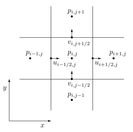
Notice how in Figure 1, that the velocity values are placed on the edges of the cells and the pressure values are placed in the center. By placing the velocity values at the edges (denoted by the \(u_{i - \frac{1}{2}}\) for the left edge and \(u_{i + \frac{1}{2}}\) for the right edge), we no longer have the issue from before when taking the derivative at the center of the cell. Namely:

$$u_i' \approx \frac{u_{i + \frac{1}{2}} - u_{i - \frac{1}{2}}}{\Delta x}$$

Notice how this does not have any missing values in between (as there we are not keeping track of the value in the cell center, \(u_i\)). Should we want the velocity at that location, we can simply interpolate the edge values.

When we compute the pressure gradient to update the velocity values, notice that we can easily use central differencing at the edges since the pressure values are kept at the cell centers.

Grid Cells

For the sake of simplicity, we'll categorize each of the cells as solid, empty/air, or fluid. This limits us to having solids that perfectly align with the grid cells and that all walls and boundaries perfectly align with the axes.

Boundary Conditions

As with every set of differential equations, Eulerian fluid simulation has several boundary conditions to consider, but the two basic requirements are the boundary between fluid and air and the boundary between fluid and solids.

Fluid-Air Boundary

The boundary between fluid and air represents atmospheric effects as well as any forces that result from wind or pressure differences. In general, air pressure is so small that it has a negligible effect and we can just ignore it.

Fluid-Solid Boundary (Normal Component)

For the boundary between fluid and solids, we first look at the normal component of the velocity field. For the 2D case, if the fluid is to the right or the left of the solid, we're looking at the \(x\) component of the velocity vector. If the fluid is above or below the solid, we're looking at the \(y\) component of the velocity vector.

Since we don't want the fluid to enter the solid cells, we want the relative normal velocity between the fluid and solid to be zero. Notice that we're dealing with the relative velocity because if the solid is moving, the fluid velocity of the fluid at their boundary can move up to the solid's velocity without entering the solid cell.

Of course, if the solid is stationary, then we set the normal velocity to be zero.

Fluid-Solid Boundary (Tangential Component)

In addition, there is also the tangential component of the fluid velocity with respect to the solid. In the 2D case, it's the non-normal direction and in the 3D case, it's both of the non-normal directions.

If we leave the tangential component alone, collisions will still not occur, and the fluid can freely travel along the side of the solids. This is called a free-slip boundary.

If we set the tangential component to zero, the fluid will completely halt upon collision and this is called a no-slip boundary.

If the boundary is set to be between the free-slip and the no-slip boundary, this is effectively the same as having a solid that's kind of sticky or one that applies a friction force on the fluid that slows it down as it travels against it.

Appendix: The Laplacian Operator

The Laplacian operator is typically written as \(\nabla^2\), but it is equivalently defined as the divergence of the gradient, \(\nabla^2 f = \nabla \cdot \nabla f\). It effectively computes how much a value varies from the average value within a small neighborhood.

A simple way to understand what the Laplacian does is to look at its discrete estimate:

$$\nabla^2 f(x, y) \approx \frac{f(x - h, y) + f(x + h, y) + f(x, y - h) + f(x, y + h) - 4 f(x, y)}{h^2}$$

Notice that when \(f(x, y)\) is more positive than its neighbors, the Laplacian is a negative value and when it is more negative than its neighbors, the Laplacian is a positive value. When it is close to its neighbors, the Laplacian is then close to zero.

From this we can see that whenever the value at a given point is far away from its neighbors, then the Laplacian at that point pushes it towards the average value. As a result, this intuitively makes sense that it corresponds with the viscosity when applied to the velocity field as it would nudge velocity values towards the local average to increase local uniformity and therefore resist deformation.

Next Time

In the next article in this series, we'll discuss how to update the state, solve constraints, and render the fluid.